Project specification
- Project title
- PyTorch Game Agent: Design, Training and Competitive Comparison
- Student
- Dávid Moniš · david5.monis@gmail.com
- Supervisor
- RNDr. Andrej Lúčny, PhD. · lucny@fmph.uniba.sk
- Topic
- Reinforcement learning and neural networks applied to playing a simple video game, with competition on Kaggle.
- Specification (Goal)
- The project is split into two consecutive phases. The first phase focuses on designing and implementing a DQN agent for the game Snake, including a complete training ecosystem in PyTorch. The second phase builds on it by extending the solution to the multi-agent Kaggle Hungry Geese environment, where the goal is to adapt the agent to the new rules and achieve measurable results in a competitive evaluation.
- Project source code
- GitHub – DavidMonis / RocnikovyProjekt
A short description of the game
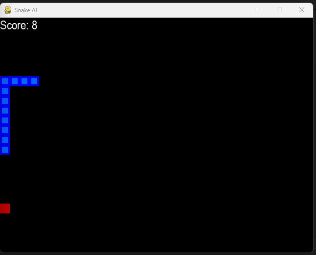
The game is a variation on classic Snake, designed as an environment for reinforcement learning. At every step the agent decides based on local information about danger, its current direction of movement and the relative position of the food. Its goal is to navigate the grid efficiently, avoid collisions with the walls and its own body, and maximize its score in the long run.
The snake's behavior is not explicitly programmed – the agent learns its strategy gradually through experience, rewards and penalties. Using Deep Q-Learning, it is able to plan its movement, adapt to its growing body length and improve its decisions as the number of episodes played increases.
The project is not just the resulting game, but a complete training ecosystem covering the definition of the state space, the action set, the design of the reward function, the neural network, the training logic, model saving and real-time visualization of learning.
What is already done
- A fully working, manually playable version of Snake built with pygame.
- A standalone RL environment with a defined state space, actions and reward function.
- A DQN neural network implemented in PyTorch (Linear_QNet).
- Training logic with separate short-memory and long-memory training.
- Saving and reloading of trained model weights.
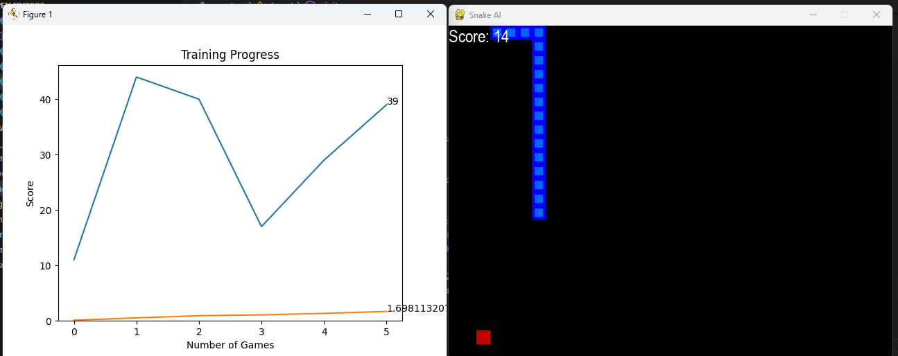
- Visualization of learning progress – score and average score over time.
- Scripts for testing and inspecting saved models.
- Generated videos comparing agents, plus a training time-lapse.
- Groundwork prepared for the extension to the competitive Kaggle environment.
Evidence and results
Below are samples of the training results. The videos show the differences between the trained agent at various stages of learning, and how training progressed over time.
Kaggle Hungry Geese
The second phase of the project replaced the DQN agent with a complete AI pipeline for Kaggle Hungry Geese – a four-player version of Snake in which a player leaving one edge of the board reappears on the opposite side. The game requires opponent modeling, long-term planning and an immediate reaction to dangerous collisions. I built my own simulator of the game environment, a CNN policy-value network, a custom MCTS and self-play training with a replay buffer.
- Self-play game generation77%
- Internal checkpoint evaluation23%
- Gradient training of the network< 1%
Fun fact: The gradient training of the network itself takes only 0.2 h of the total 65.7 h — less than 1% of the overall time. Most of it went into generating self-play games (77%) and internal checkpoint evaluation (23%). This split is typical of self-play systems, where generating data is orders of magnitude more expensive than updating the network weights.
Architecture and training
Evolution of the architecture
The final shape of the network did not appear all at once — it went through several markedly different generations. It started as a simple fully connected network with a single hidden layer, meant to verify that the model could process the input and return usable actions at all. That turned out to work, but Hungry Geese is a spatial problem — and a fully connected layer does not exploit spatial relationships efficiently.
So the architecture evolved step by step: a second hidden layer was added to capture more complex relationships, then convolutional layers (CNN) for the spatial features of the grid, and later a flatten layer after the CNN, combining the spatial features with the scalar input. The last and most important step was splitting the output part into two independent heads — policy and value — which enabled full integration with MCTS and fundamentally improved the quality of training.
Neural network
The final model is a CNN policy-value network with two output heads. It predicts both the action probabilities (policy) and the value of the current position (value), which allows it to be combined efficiently with MCTS without having to play every game out to the end.
A standalone visualization of PolicyValueNet with the real weights from the final checkpoint: 5,760 clickable nodes, the strongest connections and a step-by-step forward pass where you can see the actual numbers in every layer.
- 1,286,693 parameters
- 5,760 nodes
- 7 layers, step by step
An interactive diagram of the network. Hover over any layer (or tap it on mobile) to see its description, dimensions and parameter count.
own body · opponents' heads · opponents' bodies · opponents' tails · food · danger cells (cells an opponent's head can move into on the next step)
These values cannot be encoded into the grid — they carry the global context of the game. They enter the dense layer directly, after being concatenated with the CNN output.
Conv2d 32 → 64, 3×3, circular padding + ReLU → Flatten (4,928)
Circular padding reflects the toroidal topology of the board: the right edge is adjacent to the left one, the top to the bottom. Ordinary zero-padding would create fake “walls” at the edges that do not exist in the game. Circular convolutions model this directly — the network sees relationships across the edges of the map just as it does inside the grid.
P(N) · P(S) · P(E) · P(W)
Cross-entropy loss vs. MCTS visit counts
Position value [−1, 1]
MSE loss vs. final placement
Output heads — choosing the loss functions
The policy head predicts a probability distribution over the 4 actions: P(N) — north, P(S) — south, P(E) — east, P(W) — west. The training targets are the normalized visit counts from MCTS (so-called soft targets) — the network learns to imitate the decisions of the MCTS planning phase, not just the immediate action. For training a distribution, the natural choice is cross-entropy loss, which directly penalizes any deviation from the target distribution and is the standard for classification tasks.
The value head predicts a scalar value of the position in the range [−1, 1], where −1 corresponds to the worst placement (first one eliminated) and +1 to a win. Since this is a regression task with a single output value, MSE loss is the natural choice — it penalizes deviations quadratically, so large errors are punished much more heavily than small ones, and it works symmetrically for estimates that are too optimistic and too pessimistic alike.
Monte Carlo Tree Search
A forward pass of the network on its own is short-sighted — given the current game state it returns a distribution over actions without looking into the future at all. This is where MCTS comes in: an implicit search tree is built on top of the network, where each node represents a game state and each edge one of the possible actions.
The search is driven by the PUCT formula, which balances exploration of new branches (prioritized by the policy head) against exploitation of promising lines (based on the simulation results so far). At leaf nodes the position is evaluated by the value head — with no need to play the game out to the end. Opponents' moves inside the tree are approximated by a single policy — the NN policy during training and in the submission, and a rule-based agent during internal evaluation.
MCTS plays a double role in the project. During training it generates higher-quality training data than a purely greedy policy — the agent learns from planned decisions, not just from the network's immediate reactions. At inference it provides real lookahead, which considerably increases playing strength compared with a forward pass alone. That is exactly why splitting the network into two heads was essential: the policy head gives MCTS informed priors for selecting tree branches, and the value head evaluates positions at the leaves — together they form the basis for efficient planning without explicitly playing games out to the end. The number of simulations depends on the context: 32 when generating training games (speed), 64 for internal evaluation and 128 in the final submission (maximum playing strength within ~1 s per move).
How training progressed
Training ran in several progressively more demanding phases, with the aim of building an agent able to face a wide variety of opponents — from simple rule-based bots all the way to full MCTS agents.
Phase 1 — Foundations against bots
The first iterations were played exclusively against simple rule-based bots (stupid_bot, clever_bot, smart_bot). This was deliberate: the network first had to master basic survival, navigation and food collection before it was given stronger opponents. The results of the early iterations confirm it — the agent learned to play solidly precisely in the environment of simple bots.
Phase 2 — Gradually increasing difficulty
Stronger bots were added gradually, followed by NN agents represented by older checkpoints from previous training iterations. An important part of this was the rotation of player positions: every agent played from all 4 positions on the grid, which prevented it from learning positional biases. The share of NN agents grew steadily at the expense of the bots, but the rule-based bots never disappeared entirely — their presence prevented catastrophic forgetting of the basic strategies learned in the first phase.
Phase 3 — Self-play with MCTS
In the final phase most opponents were MCTS agents from more recent iterations, complemented by NN agents and a small share of bots. The batch size was set to 50,000 training samples. Every iteration followed a fixed order: first the whole block of self-play games was played, the new samples were added to the replay buffer, and only then did the training phase run on the updated buffer. This way, in every iteration the network learned from the freshest experience available.
This approach is effective for several reasons. Curriculum learning — gradually increasing the difficulty — ensures that the network does not start out in an environment where it receives nothing but negative feedback and has nothing to learn from. Opponent diversity prevents over-optimizing for a single type of behavior and builds a more robust strategy. Self-play guarantees that the agent always practices against an opponent of comparable strength, which is far more effective than fixed bots.
Evaluation
Internal evaluation — comparing new checkpoints against older ones — made up 23% of the total training time. The final external evaluation (a comparison against Goose Loose in three scenarios, 100 games each with position rotation) took more than 100 hours of uninterrupted running (over 4 days straight; one complete run of all three scenarios took ~36 hours on average). Reliable validation in a stochastic multi-agent game requires a large number of games so that the results are not distorted by statistical noise. Training was computationally demanding, but the most time-consuming stage of the project was the evaluation itself.
Training results
Iteration 1 — start
Iteration 102 — end
External evaluation vs. Goose Loose
The final agent was compared with the public agent Goose Loose in three scenarios of 100 games each, with position rotation.
| Scenario | Avg place (mine) | Avg place (Goose) | Win rate (mine) | Win rate (Goose) | Kaggle score (mine) | Kaggle score (Goose) |
|---|---|---|---|---|---|---|
| direct duel + 2 bots | 1.695 | 1.370 | 0.365 | 0.630 | 12,423.8 | 12,488.4 |
| balanced (2 mine + 2 Goose) | 3.168 | 1.833 | 0.153 | 0.847 | 12,650.6 | 17,144.2 |
| stress (1 mine + 3 Goose) | 3.600 | 2.133 | 0.013 | 0.987 | 11,004.6 | 17,316.3 |
Avg placement: lower = better (1.0 = first place). Win rate includes shared wins and is normalized by the number of games, not by the number of agent copies.
The results confirm that Goose Loose consistently outperforms my agent in all three scenarios. The gap widens in proportion to the share of Goose Loose agents in the game: in the direct duel scenario both compete primarily against weaker rule-based bots, which leads to closer placements (1.695 vs 1.370). In the balanced scenario Goose Loose agents replace both bots and the competitive pressure doubles — my agent's average placement drops to 3.168. In the stress scenario a single copy of my agent faces three copies of Goose Loose; for any single agent facing three stronger opponents at once, a placement close to 4.0 is the statistically expected outcome — my agent achieved 3.60. The Kaggle score (the raw reward encoding steps survived and body length) confirms the same trend: while Goose Loose keeps consistently high values across all scenarios, my agent's score drops sharply in the stress scenario, which reflects shortened survival rather than a worse quality of play.
Game demos – Hungry Geese
Recordings of the final agent's games in various game scenarios, captured locally with a pygame visualizer.
Agent evolution — 4 iterations at once (Games 1–4)
Four windows at once — same seed, same opponents (clever: 1 (green), smart: 2 (yellow), stupid bot: 3 (pink)), different iteration. Top left: iter_0010 · Top right: iter_0030 · Bottom left: iter_0060 · Bottom right: iter_0100. You can see how, with each iteration, the agent learns to survive longer and react better.
Final agent vs. Goose Loose (Game 5)
The final MCTS agent (submission.py) in a head-to-head duel with the strong public agent Goose Loose. This is the closest variant to the real Kaggle evaluation. stupid_bot: 0 (blue) · smart_bot: 1 (green) · MCTS: 2 (yellow) · Goose Loose: 3 (pink).
MCTS vs. NN agents (Game 6)
One MCTS agent (submission.py) against three cheap NN agents without tree search. Both sides use the very same neural network — the only difference is whether the network gets time for MCTS or decides with a direct forward pass. MCTS: 0 (blue) · NN direct: 1 (green) · NN direct: 2 (yellow) · NN direct: 3 (pink).
MCTS vs. MCTS (Game 7)
Four copies of the final agent play each other — a pure self-play scenario. All four use full MCTS with 128 simulations. The game shows how the agent behaves when facing equally strong opponents. MCTS: 0 (blue) · MCTS: 1 (green) · MCTS: 2 (yellow) · MCTS: 3 (pink).
Conclusion
The final MCTS agent was not able to beat Goose Loose — an agent that won a gold medal in the Kaggle Hungry Geese competition and was developed by a team of 5 experienced specialists. But when I look at the financial, knowledge and time resources I had at my disposal, the result is remarkably close to what an expert group with far greater infrastructure produced. This project shows how far you can get with a rigorous methodology, even when working alone and with limited means. Despite the scale of the project — 4,754 lines of production code in 24 files, 5,406 lines of tests in 18 test files, 13,400 lines in total — it was not enough to beat expert solutions backed by more computing capacity and years of experience.
The most valuable outcome is not the agent's performance itself, but an understanding of the whole process: designing the architecture and choosing loss functions, curriculum learning and self-play dynamics, integrating MCTS with a neural network, evaluation methodology in a stochastic multi-agent game — these are skills and experience transferable far beyond this particular competition. The project also showed how fundamental the difference is between a working agent and a truly top-tier competitive solution: a good idea is not enough, it takes computing power, large amounts of data, precise simulation and long-term tuning of every detail.
Where next
The project has a natural continuation in game AI: another Kaggle competition, in which the experience gained — the training infrastructure, the evaluation approach, the evolution of the architecture — would be a solid starting point compared with starting from scratch.
A more interesting and, today, more practically relevant direction is a move towards the dominant area of current machine learning: large language models (LLMs). Open-source models such as Llama or Qwen open up the possibility of doing my own fine-tuning — adapting a pre-trained model to a specific task or domain. The knowledge gained in this project transfers directly: an understanding of training dynamics, the importance of data quality and diversity, the design and combination of loss functions, evaluation discipline and the systematic repetition of experiments. All of these principles apply just as much to training a game agent as to fine-tuning a language model.
It would be a natural and logical step: from the fun, game-playing side of neural networks to what is today the most widely used and most popular area of AI — and with the foundations this project has provided, such a move would be far less steep than it seems at first glance.